Stern–Gerlach · spin is quantized in space

When a magnetic moment is sent through an inhomogeneous field, can it point any direction (a continuous smear on the detector) — or only a discrete set of directions?

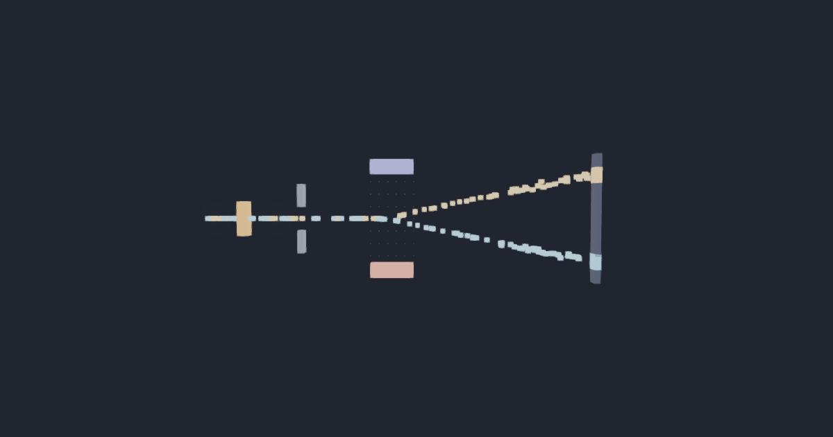
▶ Run the simulationSee the measured result

Units: J/T (Bohr magneton μ_B)

How the lab tests it

Send a velocity-selected beam of silver atoms (one unpaired electron ⇒ net moment ≈ one Bohr magneton) through a field gradient G = ∂B_z/∂z. The force on a moment is F_z = μ_z·G, so each atom deflects by z = μ_z·G·L·(L/2+D)/(M v₀²) (a parabola through the magnet of length L, then a straight drift D to the detector). Forward-model two populations of 4000 atoms — quantum (μ_z = g_s·m_s·μ_B, m_s = ±½) and a classical control (μ_z = μ_B·cosθ, cosθ isotropic) — with a velocity passband and detector noise, seeded → reproducible. Measure the central-gap fraction and the mean deflection.

What it checks

the spin quantum number s = ½ and the electron magnetic moment of one Bohr magneton (g_s ≈ 2). The beam does NOT paint a continuous band — it splits into exactly TWO spots, so 2s+1 = 2 ⇒ s = ½. The classical isotropic moment fills the centre (central-gap fraction ≈ 0.4); the quantum beam leaves a clean dead zone between the spots (≈ 0). From the mean deflection the lab recovers the Bohr magneton WITHOUT being told it: μ_B = ⟨|z|⟩·M·v₀²/(G·L·(L/2+D)) ≈ 9.27×10⁻²⁴ J/T, giving g_s = 2μ_z/μ_B ≈ 2 — twice the value orbital angular momentum would give, the anomaly that pointed at electron spin. Stern & Gerlach's 1922 result (Nobel 1943) — the first direct proof of space quantization and the eighth pillar of early quantum theory after Millikan's charge

Stern–Gerlach deflection & Bohr magneton calculator

What a beam of atoms does to a magnet that is stronger at one end than the other, and what falls out of the answer. A uniform field only turns a magnetic moment; a GRADIENT pulls on it, with a force μ_z·∂B_z/∂z that depends on which way the moment points — so the detector spot is a readout of orientation. Classically the moment could point anywhere, and the beam should arrive as one continuous smear filling the centre; it arrives as two separate spots with a clean dead zone between them, and that dead zone is the whole 1922 result. Every number here is built from what you type: μ_B is assembled as eħ/(2mₑ) rather than stored, which is the same refusal that makes the simulation above non-circular — it reads the moment back off the detector through the beam speed and the geometry alone, and μ_B enters only the atoms it simulates and the final score. The measured-deflection box defaults to 1.9647169 mm, and that is deliberate: it is this lab's own 4000-atom draw, not the textbook figure, so inverting it hands back 9.329605×10⁻²⁴ J/T — the +0.60% the on-screen HUD discloses — and dividing out the ±4% velocity passband lands it on (g_s/2)μ_B to 0.003%, which is how that offset is known to be two named systematics rather than noise. Four things this lab does not measure, so the calculator does not pretend to: the actual field of a real pole pair, which is never a single number G but a map with a transverse gradient attached; the finite beam width and oven collimation that decide whether two spots are resolvable at all, and very nearly sank the 1922 run; the hyperfine and nuclear moments, three orders of magnitude smaller, that a modern apparatus resolves inside each of these spots; and the quantum measurement problem itself — this page computes where the spots land, never why a single atom picks one.