Wave interference

When two coherent wave sources overlap, do they interfere — and does the pattern obey the wave equation's dispersion relation?

▶ Run the simulationSee the measured result

How the lab tests it

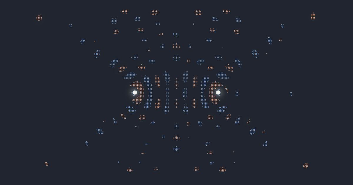
Drive two in-phase point sources on a 2-D membrane (the wave equation ∂²u/∂t² = c²∇²u, absorbing borders), watch their circular waves overlap, and measure the wavelength λ from the field's spatial autocorrelation.

What it checks

interference — bright bands where the paths differ by a whole wavelength, dark nodal lines where they differ by a half — and the dispersion relation c = λ·f (the measured phase speed matching the model's wave speed)

Courant (CFL) number, stability limit, numerical dispersion & grid-resolution calculator

A simulation of a wave is not a wave, and the difference is a number you can write down. The membrane above knows one rule -- u(n+1) = 2u(n) - u(n-1) + C^2 times the five-point Laplacian -- and everything anybody wants from it follows from the single dimensionless group in that line, the Courant number C = c*dt/dx. It decides two things that pull against each other. Too large and the scheme does not merely lose accuracy, it explodes: one Fourier mode turns the update into a quadratic whose roots multiply to 1, so the pair either sits on the unit circle or one root escapes it, and the escape happens the instant C^2*d exceeds 1. That is the CFL condition, and the limit is one square root, 1/sqrt(d) -- 1 in a line, 0.707 on a plane, 0.577 in a volume. Too small and the grid lies about the speed of light in its own medium. The lattice does not obey omega = c*k; it obeys sin(omega*dt/2) = C*sin(k*dx/2), von Neumann's discrete relation, of which the continuum law is only the small-argument limit. Drive this lab's grid at 13 cells per cycle and the wave that comes back is 12.9033 cells, short by 0.744%, and that deficit is not noise: the simulation above measured 12.9012 +/- 0.0014 across eight seeds and the closed form on this page predicts it to one part in six thousand, while lambda = c/f -- the formula in every textbook -- is out by seventy-five standard errors on the same data. Nothing here is stored. Every wavelength, limit, phase error and node spacing below is assembled from the boxes, and this lab's own readings are carried only to be scored against. Three consequences of that one relation are worth the page on their own. The error carries a factor (1 - C^2), so the most ACCURATE time step is the largest stable one -- the opposite of nearly every other integrator, and at C = 1 in one dimension the scheme is exact at every wavelength. In two dimensions a square grid is not a square of space: the diagonal and the axis disagree, and at C = 1/sqrt(2) the diagonal becomes exactly dispersion-free while the axis does not. And the design rule everybody actually uses falls out of a third-order expansion: N = pi*sqrt((1 - C^2)/(6*error)) cells per wavelength, which is where 'ten cells per wavelength' and 'twenty cells per wavelength' come from. Four things this page will not do. It will not give a wavelength at a general propagation angle, because sin(omega/2) = C*sqrt(sin(kx/2)^2 + sin(ky/2)^2) has no closed-form inversion off the axis and the diagonal, and inventing one is exactly what a page under a finding may not do. It will not model amplitude -- node DEPTH needs the geometric decay this lab simulates and this page does not. It will not do the far-field double slit, which is ?world=young's phasor sum with no medium in it, a different limit and not this formula rearranged. And it will not correct a number the lab recovered, including the shipped module's own on-screen 13.5 cells, whose 4.9% offset the finding locates in a measurement stride and gates there.