Galton board · Central Limit Theorem

Why is the bell curve everywhere? If you sum many independent random ±1 steps, does the result always become Gaussian — and how fast?

▶ Run the simulationSee the measured result

Units: dimensionless (log–log convergence exponent of the symmetric board's pointwise gap; secondary knowns: −1 biased, −1/2 CDF, amplitudes φ(0)/2 = 0.1994711 and φ(0) = 0.3989423, Edgeworth prefactor M|1−2p|/(6pq) with M = 0.54763, Lévy exponent 1/α = 2/3)

How the lab tests it

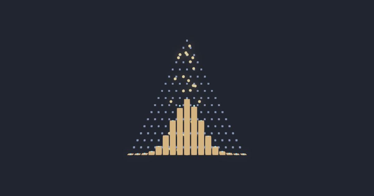
Drop thousands of balls through n rows of pegs (each a ±1 Bernoulli step with probability p); the count of rights is a sum of n independent steps, binned into a histogram with the exact Gaussian N(np, np(1−p)) overlaid. A separate exact experiment plots the maximum pointwise gap Δ(n) between the binomial and its Gaussian limit, log-log, across n = 4…256.

What it checks

the CLT: the histogram fills the bell with measured mean → np and standard deviation → √(np(1−p)); and the convergence RATE — Δ ∝ n^(−3/2) for a symmetric board (the leading skewness correction vanishes at p=½), slowing to Δ ∝ 1/n once the board is biased (p≠½)

Galton board & binomial calculator (mean, spread, and how fast the bell curve arrives)

The oldest limit theorem in probability, priced rather than quoted. Balls fall through n rows of pegs, turn right with probability p at each one, and pile up into a bell curve — de Moivre in 1733, Laplace in 1812, the first central limit theorem there was. What this page computes is not that the pile is Gaussian but HOW FAR IT IS FROM BEING ONE, and that gap has a closed form nobody has to fit. Nothing here is stored: the mean is assembled as n·p and the spread as √(npq) from the two numbers you type, the exact bin heights come out of the two-point kernel's own ratio recursion — no factorials, no binomial coefficients, nothing raised to a power — and the Gaussian they are scored against is φ(0) = 1/√(2π) times an exponential this page BUILDS out of its own series instead of calling. So there is no implementation-approximated function anywhere on it, every figure is the same double in every browser, and the de Moivre–Laplace gap is computed here rather than copied. THE INTERESTING NUMBER IS AN EXPONENT, AND THERE ARE THREE OF THEM. On a fair board the pointwise gap dies as n^(−3/2); load the board and it dies only as 1/n; and the cumulative gap dies as n^(−1/2) on both. One counted distribution, three different speeds, and the reason is which Edgeworth term survives — a symmetric board has γ₁ exactly zero, so the skew term is not small but ABSENT, and symmetry alone buys half a power of n. The amplitudes are parameter-free too and this page derives them rather than looking them up: at the centre the skew term carries He₃(0) = 0 whatever p is, so what is left collapses to φ(0)(1−pq)/(12(pq)^(3/2)), which at p = ½ is the φ(0)/2 = 0.1994711 the finding recovers as 0.199465 — and off centre the constant is the sup of |He₃φ|, which sits at the exact surd x* = √(3−√6) and needs no root-finder. Fed this lab's own doubling rung the page returns −1.49995593 on a fair board and −1.00190377 on a loaded one, against the −1.49996 and −1.0019 the world measured by exact convolution. The rival is a dial rather than a name: 'enough addition always makes a Gaussian' is false, and α is the step law's tail exponent — below 2 the width grows as n^(1/α) and the limit is Lévy rather than Gaussian, at 2 and above the variance is finite and the dial hands the board's own √2 per doubling back as the same double. Three things this page will NOT do. It will not price a binomial probability as an end in itself — the exact heights are an ingredient here, and the random-geometric-graph page on this site is where C(n,k)p^k q^(n−k) is the answer. It will not evaluate the normal CDF: locating the cumulative sup needs an error function, and one call would cost every figure here its cross-engine guarantee, so the lattice FLOOR is computed and the sup is left to the oracle. And it will not correct a single number the finding recovered: it prices closed forms, and the measured values belong to the simulation above.