Parallel LC tank · antiresonance

Take the same coil, capacitor and resistor from the series RLC world, but wire them in PARALLEL and push a fixed AC current through them. Does the tank still 'prefer' ω₀ = 1/√(LC) — and does it respond the same way the series loop did, or the opposite?

▶ Run the simulationSee the measured result

Units: Hz — f₀ = 1/(2π√(LC)) of the real tank (250 µH · 100 pF), the same Thomson frequency as the series loop, in the AM broadcast band

How the lab tests it

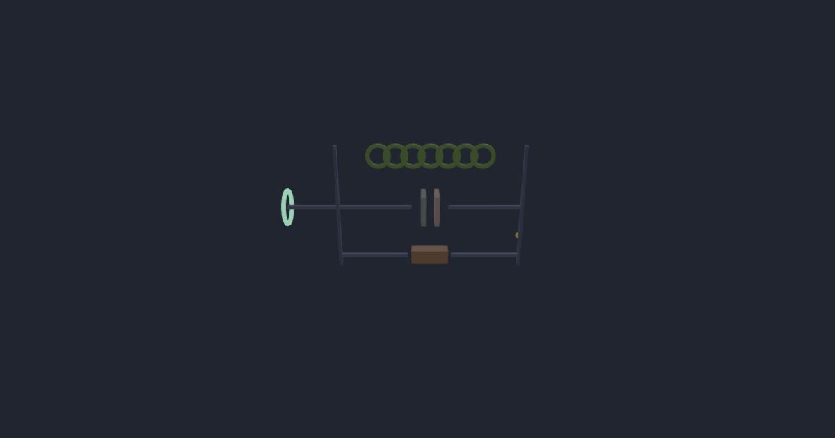
Drive a parallel L‖C‖R tank with a fixed-amplitude current source I₀cos ωt, so its admittance is Y = 1/R + j(ωC − 1/ωL) and its impedance |Z|(ω) = 1/√((1/R)² + (ωC−1/ωL)²). The lab sweeps the drive frequency through ω₀ and traces |Z|(ω), shading the half-power band, while the live coil (½LI_L²) and capacitor (q²/2C) hand the energy back and forth and a pulse races the circulating current round the L↔C loop. The same AM tank — L=250 µH, C=100 pF — is read as a parallel resonator with loss R_p≈250 kΩ and swept with ±1.5% reading noise.

What it checks

It is the exact DUAL of the series loop. The impedance |Z| PEAKS sharply at ω₀ = 1/√(LC) (where it dipped before), so a fixed drive current produces a huge node voltage there and the tank looks like a bare resistor R — antiresonance. The sharpness flips to Q = R√(C/L) = ω₀R_pC, so a BIGGER R now sharpens the tank (it damped the series one). And at ω₀ the two branch currents are equal and opposite, nearly cancelling at the source: a current Q·I₀ circulates in the L↔C loop while the source draws only I₀ (current magnification). A high impedance at ω₀ BLOCKS that frequency in a line — the parallel tank is the band-stop 'trap' and the oscillator's frequency-setting resonator, the mirror of the series tank that PASSES ω₀. Reading the real tank recovers f₀ ≈ 1.01 MHz and Q ≈ 158 — and that same Q is the current magnification I_circ/I₀ ≈ 158×

Parallel LC tank — antiresonance, the impedance peak at R_p, current magnification & wave-trap depth

The same coil and capacitor as the radio's series loop (?world=rlc), wired in PARALLEL, and almost every sign turns over. The frequency does not: f₀ is still 1/(2π√(LC)), Thomson's 1853 number, which is why this page assembles it from the same two parts and reads no resistance at all. Everything else dualises. The impedance PEAKS here where the series loop DIPS, and it peaks at the bare loss resistor R_p. The quality factor carries that resistor in the NUMERATOR — Q = R_p√(C/L) — so a BIGGER loss resistance makes a parallel tank SHARPER, the exact opposite of the series law Q = √(L/C)/R, and this is the single most counterintuitive line on the page. Nothing here is stored: f₀ is assembled out of the two parts you type, Q as R_p divided by the characteristic impedance √(L/C), and the lab's own readings are carried for SCORING only — zero every one of them and not a single computed number moves. The defaults are this world's bench, the AM tank of 250 µH and 100 pF read in parallel with R_p = 250 kΩ: f₀ = 1006584.2421 Hz, Q = 158.113883, half-power width 6.366198 kHz, impedance peak 250 kΩ. The simulation above reaches that frequency down a different road — it integrates Kirchhoff's node equations C·v̇ = I₀cos ωt − v/R_p − i_L and L·i̇_L = v and bisects the drive frequency at which the node voltage comes into phase with the drive current, with no 1/√(LC), no impedance formula and no Q anywhere in its recovery — and its 24-seed noisy read of 1006588.9 ± 7.5 Hz lands 0.621055 bars from the closed form, which is the only reason the agreement is worth anything. Three things here are second routes rather than restatements. Q arrives a THIRD way, from energy: 2π times the energy stored at the voltage peak divided by the energy dissipated per cycle returns 158.113883 through arithmetic containing neither √(C/L) nor any bandwidth — the definition of Q, closing on the parts-list formula. The finding asserts that a current Q× the supply circulates in the L↔C loop and never says what voltage that implies; it is 250 V standing across a tank fed 1 mA, because at resonance the tank looks like its own 250 kΩ. And the duality dictionary is priced in both directions: the equivalent series loss R_s = L/(C·R_p) = 10 Ω and the return trip R_p = Q²·R_s = 250 kΩ, which is how one physical coil is read two ways. Four things this page will NOT do. It will not re-run the simulation above. It will not model a real coil or capacitor — no winding resistance, core loss, self-capacitance or skin effect, no dielectric loss — every one of which drains the tank and so LOWERS the effective R_p, which makes the Q below a CEILING on sharpness rather than a promise. It is the PARALLEL tank and not the series loop, whose extremum is a minimum of impedance rather than a maximum. And it will not correct a single number the finding recovered: it prices closed forms, and the measured values belong to the oracle.