Resonance · the driven oscillator

Push a damped mass-on-a-spring at frequency ω — how big a swing do you get, and how far behind does it lag?

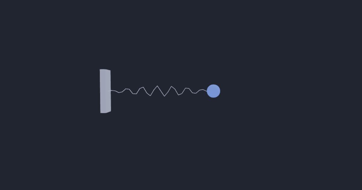
▶ Run the simulationSee the measured result

Units: dimensionless (ω_r/ω₀ at Q = ω₀/γ = 4; exactly √(1 − γ²/(2ω₀²)) = √(31/32))

How the lab tests it

Drive a damped oscillator (ω₀=2, γ=0.5) with F=f₀·cos(ωt). At each ω wait out the transient, then LOCK IN: integrate x·cos(ωt) and x·sin(ωt) over whole drive periods — the two quadratures recover the steady amplitude A and the phase lag φ at once. Sweep ω across ω₀ and overlay the measured (A,φ) on the analytic curves.

What it checks

the Lorentzian A(ω)=f₀/√[(ω₀²−ω²)²+(γω)²], peaking at the resonant frequency ω_r=√(ω₀²−γ²/2) with sharpness Q=ω₀/γ, and the phase lag φ=atan2(γω, ω₀²−ω²) that sweeps 0→π and passes through EXACTLY π/2 at ω=ω₀. Measured points land on the Lorentzian to 3–4 digits; the peak (1.97 vs 1.969) and the φ=90° crossing (2.00 vs ω₀=2.0, damping-independent) hit to ~0.05%, with A_max and Q a few % low only because the drive grid is coarse near the peak

Resonant frequency, Q factor & half-power bandwidth calculator

Three different frequencies are called “the resonant frequency”, and at any damping you can actually measure they are three different numbers. A driven damped oscillator ẍ + γẋ + ω₀²x = f₀cosωt has a natural frequency ω₀ that it never resonates at, a free ringdown ω_d = √(ω₀−γ²/4) that it oscillates at when nobody is driving it, and a displacement-amplitude peak at ω_r = √(ω₀²−γ²/2), which is the one a resonance curve actually shows you. This calculator assembles all three from one subtraction — ω² = ω₀² − r·γ² — and r is the only dial that separates them: 1/2 is the amplitude peak, 1/4 is the ringdown, and 0 is the textbook slogan “it resonates at its natural frequency”, which is the rival the simulation above falsifies. No resonant frequency is stored anywhere on this page. Two markers do NOT move with damping and the page computes both: the phase lag crosses 90° exactly at ω₀ for every γ, and the velocity amplitude peaks exactly at ω₀ with the tidy height f₀/γ — which is why a velocity pickup and a displacement pickup on the same rig disagree about where resonance is, and both are right. There are also two thresholds rather than one: the amplitude peak disappears at γ = √2·ω₀ (Q = 1/√2), while the oscillator keeps ringing until γ = 2ω₀ (Q = 1/2), so there is a whole band of oscillators that ring and do not resonate. The Q factor is two numbers as well: the half-power bandwidth solves a quadratic in ω² whose discriminant collapses to γ²(4ω₀²−γ²), and the Q_FWHM = ω₀/Δω it returns tends to ω₀/γ only as the damping vanishes — at Q = 4 the two are still 1.6% apart, which is the gap the module above prints on screen instead of reconciling. The inverse direction is the one an experimentalist needs: from a measured peak ratio ρ = ω_r/ω₀ it solves γ = ω₀√(2(1−ρ²)) and propagates the error bar through the subtraction, which costs you four orders of magnitude — a ratio known to eleven figures buys a damping known to nine. Four things this page will not do: fit a Lorentzian, correct any number the simulation recovered, treat the band midpoint as a centre frequency, or pretend the two Q's are the same quantity.