Bak–Sneppen evolution · self-organized criticality

The sandpile drove itself critical with no tuned knob. Does the same happen in EVOLUTION — does an ecosystem self-organize to a critical state, and does extinction come in scale-free bursts?

▶ Run the simulationSee the measured result

How the lab tests it

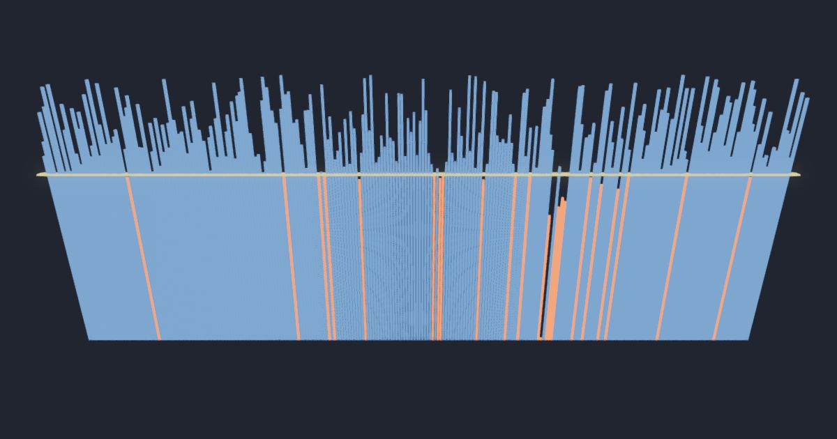
Run the Bak–Sneppen model: a ring of N=256 species each with a fitness f∈[0,1]; each step the LEAST-fit species and its two ring neighbours go extinct and are replaced by fresh random fitnesses. With no tuned parameter, accumulate the stationary fitness histogram and measure the self-organized threshold f_c two ways — the half-height edge of the histogram, and 2⟨f⟩−1 (the stationary fitnesses are ≈uniform on [f_c,1]).

What it checks

self-organized criticality with no knob: the fitnesses pile up above a sharp threshold f_c ≈ 0.667 (the 1-D nearest-neighbour Bak–Sneppen value), and evolution proceeds by PUNCTUATED EQUILIBRIUM — long calm spells above f_c broken by sudden scale-free 'coevolutionary avalanches' of extinctions (the same SOC signature as the sandpile, here as mass-extinction bursts). f_c is a precise numerical (not closed-form) value; the finite-N live estimate carries a small finite-size correction

Bak–Sneppen self-organized criticality calculator

Self-organized criticality is the claim that a system can tune ITSELF to a critical point with nobody turning a knob, and the Bak–Sneppen ring is the cleanest place to test it: kill the least-fit species and its two neighbours, replace all three at random, repeat forever. There is no parameter in that rule — and yet the ecosystem climbs to a sharp barrier threshold f_c and stops there, with its survivors spread uniformly above it, which is what makes every box below computable from a single number. That threshold has NO closed form; it is a numerically-determined constant, so this page refuses to type it in. f_c is an editable field defaulting to what this lab's own screen reads (0.64641, honestly low), the string 0.667 appears nowhere in this calculator's code, and the literature value arrives only as an OUTPUT — recovered backwards, twice, by dividing the two numbers the simulation above displays by the two biases its finding discloses, which return 0.667021 and 0.667048 from readings of 0.64641 and 0.62956. Everything else here is exact: the stationary plateau ρ = 1/(1−f_c) and mean ⟨f⟩ = (1+f_c)/2 and their two inversions, which agree only if the field really is a step; the mean-field rival, where a one-line balance — K fresh barriers per step deposit K·f_c below the threshold and exactly one is removed — gives f_c = 1/K exactly, hits this lab's random-neighbour control at 0.3319 within 0.43%, and then FAILS by a factor of two on the 1-D ring, which is the whole difference between mean field and space; and the punctuated-equilibrium test, where a largest-to-mean ratio of 78.6 leaves an exponential process expecting 1.06e-30 such bursts. The last direction is the one worth reading if you build instruments: it tests a displayed number for GRID-LOCK against the histogram it came from, because this world's own screen was caught returning a bin centre — exactly 0.6625 at N = 256, 512 and 1024 alike — a readout that looked 0.7% accurate precisely because the snap nearly cancelled the finite-size deficit, and carried no information about the system at all. Three things this lab does NOT measure, so the calculator does not pretend to: the avalanche exponent τ is read off a survival slope rather than fitted with a cutoff, so it is a definition here and not a determination; the finite-size extrapolation to f_c is not attempted, because at N = 1024 the trend is already noise-limited; and nothing on this page knows why 0.667 is 0.667 — no closed form exists, which is exactly why it is a box rather than a constant.