Soliton train · KdV inverse scattering

What happens to an arbitrary pulse under the KdV equation — does it just disperse into noise, or does its eventual fate already encode a specific set of solitons at t=0?

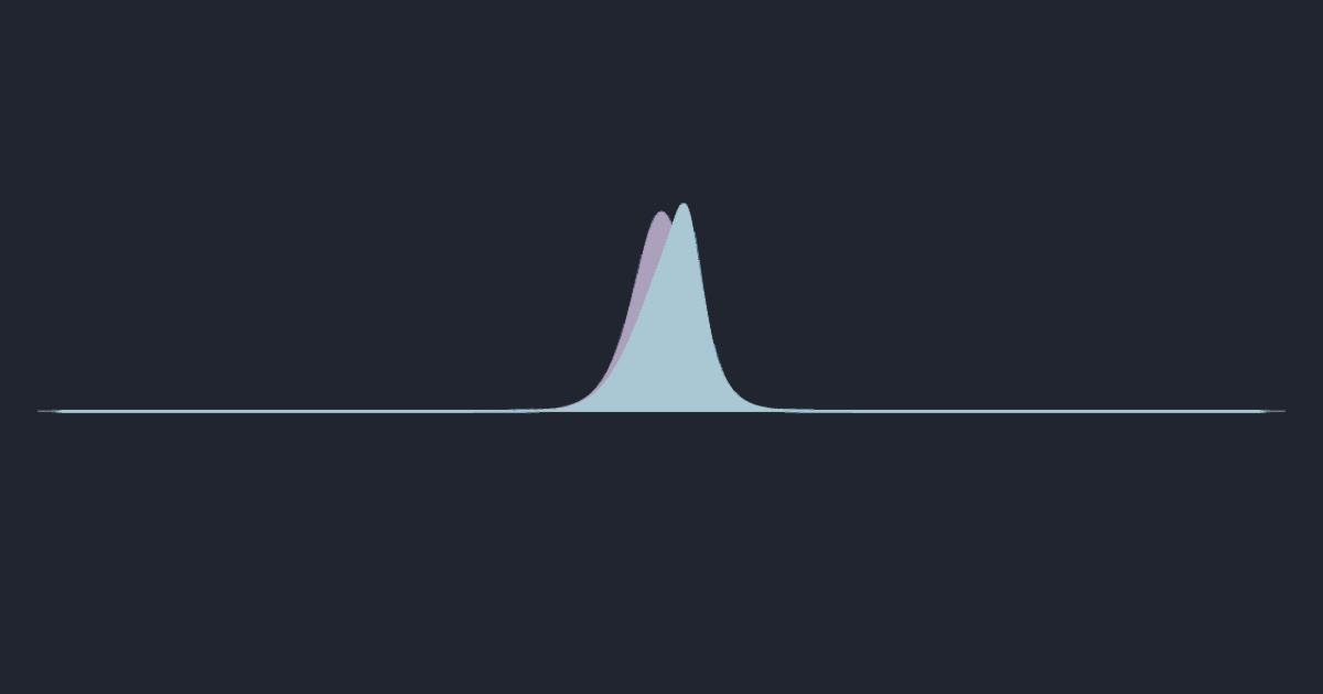
▶ Run the simulationSee the measured result

Units: dimensionless amplitude (a₃ = 2(Nλ)² for N = 3, λ = 0.4 — the tallest bound state of the Pöschl–Teller potential, GGKM 1967)

How the lab tests it

Integrate the KdV equation u_t + 6u·u_x + u_xxx = 0 (the same Zabusky–Kruskal leapfrog as the soliton world) starting from a reflectionless pulse u(x,0)=N(N+1)λ²·sech²(λx) — here N=3, λ=0.4. Let it evolve until the humps separate, then measure each emergent soliton's height and spatial order, comparing to the inverse-scattering prediction a_n=2(nλ)².

What it checks

inverse scattering (Gardner–Greene–Kruskal–Miura, 1967): the pulse sorts itself into EXACTLY N solitons — no leftover dispersive ripple for the reflectionless pulse — with quantized heights a_n = 2(nλ)², the bound-state spectrum of the Schrödinger operator whose potential is the initial pulse. The N=3 bump (height 1.92) splits into three solitons of heights 2.88 / 1.28 / 0.32 — a clean 9 : 4 : 1 (the squares 3² : 2² : 1²) — rank-ordered with the tallest in front (taller = faster, c = 2a). The soliton content is fixed at t=0; evolution merely unpacks it.

Soliton fission calculator — the bound-state count, the quantized 2(nλ)² spectrum, the amplitude thresholds, and what the radiation carries away

Drop any lump into shallow water and it does not stay one lump. It breaks into a procession of solitons, tallest in front, and the number in that procession is an INTEGER fixed at the instant you let go — before the pulse has moved at all. That is the part worth sitting with: a continuum equation with no integers anywhere in it answers a question whose answer is 3. The count is the number of bound states of a quantum well shaped like the pulse you dropped, because the KdV equation's hidden linear problem is Schrödinger's, and a sech² well is the one every quantum textbook solves exactly. So this page computes a count, a quantized ladder of heights, the thresholds at which a pulse becomes tall enough to make one more soliton, and the conserved totals the leftover radiation has to carry. Nothing it is about is typed into it. Two things are declared — the profile's sech² shape and the ladder κ_n = (ν−n+1)λ — and everything else is assembled: the two shape moments are Simpson-integrated in your browser rather than quoted, so the mass and energy sum rules are checked and not asserted, and the inversion direction hands back ν ≈ 3 from two measured wave heights without either the 3 or the λ ever being entered. The three measured-amplitude boxes hold this lab's OWN on-screen readings rather than textbook values, which is why that free inversion returns 2.989, 2.997 and 3.000 from the three pairs instead of a clean integer — the O(Δx²) mesh bias the finding prices rather than hides. Five things this page will NOT do, because the lab does not measure them. The single soliton's speed law, its width law and the two-soliton phase shift are a different page (?world=kdv) and a different question — this one never asks what a soliton DOES, only how many of them a pulse contains and how tall each is; it reports c = 2a where the ordering needs it and sends you there for why. It will not give the radiation a SHAPE: the two conserved remainders below are exact and the tail's actual profile is an Airy-type integral this lab never measured. It will not carry a number into a real channel — everything lives in the scaled frame the equation is integrated in, and a wave tank needs the shallow-water scaling that no gate here tests. It has no dissipation, so nothing in the procession ever dies. And it is one-dimensional: the transverse instability that breaks a real crest into segments is out of scope entirely.