Predator–prey

Do predator and prey populations settle to a balance, or oscillate forever?

▶ Run the simulationSee the measured result

Units: dimensionless population — the prey time-average ⟨x⟩ = γ/δ = 2.0 and predator time-average ⟨y⟩ = α/β = 2.0, both equal to the coexistence fixed point; secondary knowns: small-amplitude period T₀ = 2π/√(αγ) = 2π, culling law ⟨x⟩ = (γ+m)/δ

How the lab tests it

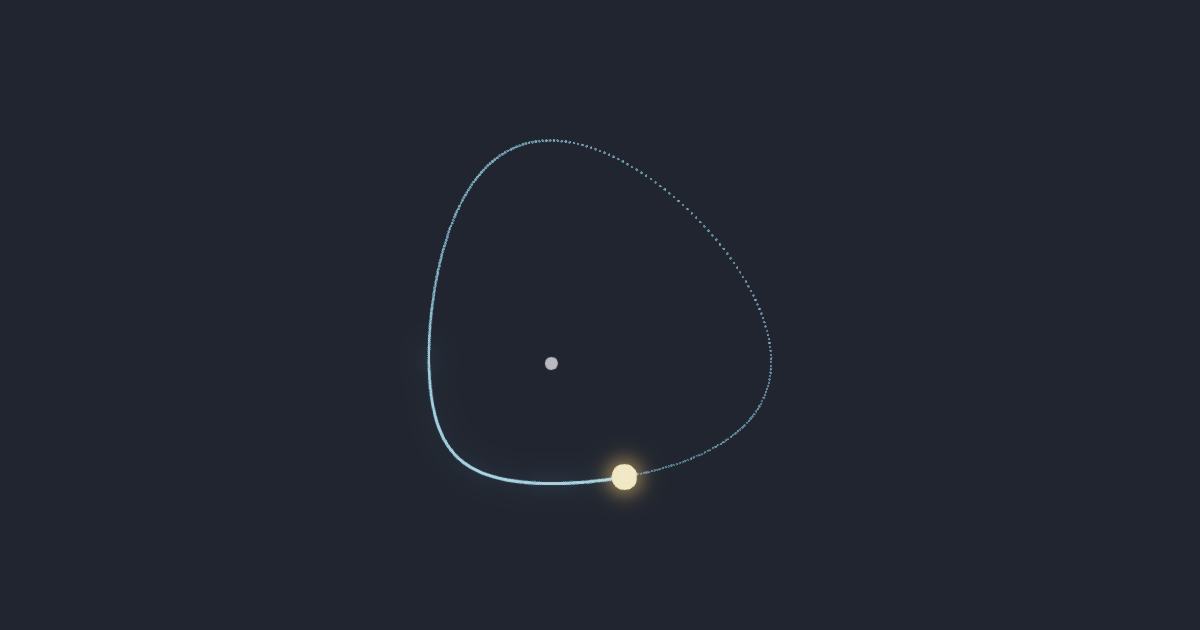
Integrate the Lotka–Volterra equations (RK4) and watch the phase-space orbit; track the conserved quantity V and measure the cycle's period from successive prey peaks.

What it checks

a closed orbit (V = δx − γ·ln x + βy − α·ln y conserved) with small-amplitude period T₀ = 2π/√(αγ)

Lotka–Volterra predator–prey calculator (fixed point, period, boom–bust range, Volterra's principle)

Two rate laws with four coefficients, and populations that neither settle nor explode. Nothing on this page is stored: every number is ASSEMBLED from the four rates you type. The coexistence point is x* = γ/δ and y* = α/β, and Volterra's law of averages (1926) is the non-obvious part — the TIME-AVERAGE of each population over a cycle sits EXACTLY on that point, at any amplitude, however wildly the boom–bust swings. The small-amplitude period is T₀ = 2π/√(αγ), and the surprise there is what is missing from it: β and δ, the two interaction strengths, do not appear at all, so how hard the predators graze sets the SIZE of the cycle and nothing about its clock. At this lab's bench — α = 1, β = ½, γ = 1, δ = ½ — that is (2, 2) and exactly 2π. THE BOOM–BUST RANGE IS WHERE THIS PAGE EARNS ITS KEEP, and it is the one thing the finding never computes. Every orbit is a level curve of V = δx − γ ln x + βy − α ln y, so its excess above the fixed point is c = γ·h(x₀/x*−1) + α·h(y₀/y*−1) with h(1+w) = w − ln(1+w); the prey's extremes are then the TWO roots of h(1+w) = c/γ, one below the fixed point and one above — the two real branches of the Lambert W, reached here by a series reversion in √(2c) polished by Newton, worst 2.87e-16 over thirteen decades of c. Released at the module's own (1, 1) the prey runs between 0.71480591236277791 and 4.3065847282206988, a 6.02× swing whose ARITHMETIC MIDPOINT is 2.5106953202917386 — 25.53% above the mean. That is the falsified rival, and it stops being a demonstration and becomes arithmetic: the lab measured its midpoint at 2.014, 2.066, 2.149 and 2.253 across four orbits, and the closed form above returns all four within their own printed rounding, without integrating anything. In the small-amplitude limit the bias has a closed form of its own, 2c/3γ, which is why the rival is not merely wrong but wrong BY AN AMOUNT THAT GROWS WITH THE CYCLE — it is not even a fixed number, while the true mean never moves. THE SPELLING OF h IS A MEASURED CHOICE, not a stylistic one. Written the textbook way, u − 1 − ln u, it loses relative precision without bound as the orbit shrinks — 1.29e-4 wrong at w = 1e-12, where the answer is 5e-25 — and Math.log1p does NOT rescue it: measured against that truth the two spellings have the IDENTICAL worst case, 9.236e-8, at the IDENTICAL argument, and return the same relative error on 99.86% of 22390 random w — log1p is strictly better on 0.08% of them and fixes nothing, because the cancellation lives BETWEEN w and log(1+w) rather than inside the logarithm, which is the reverse of the usual reflex. The cure is to never form the difference: h(1+w) = w²/2 − w³/3 + w⁴/4 − … , and the band where that series actually wins was measured at |w| ≤ 0.3, not guessed — above it log1p is the better of the two and this page uses it, at its own default release included. A hand-built logarithm was measured first and LOST to the engine's by sixfold, so the engine kept the job. One consequence runs through everything here: the orbit is carried as w = x/x* − 1 and never as x/x*, because storing 1 + w in a double discards w's low bits for any small cycle — a reference built the other way reported this page's own inversion as 2.5e-11 wrong when it was correct to the last bit. Three things this page will NOT do. It will not give you the finite-amplitude period: T₀ is the amplitude → 0 limit, real cycles are SLOWER, and that dependence has no elementary closed form — the lab measures it, and a formula offered for it here would be an invention. It is the undamped, carrying-capacity-free Lotka–Volterra only: give the prey a logistic ceiling and the conserved quantity dies, the orbit spirals in, and the law of averages stops being true. And it will not correct a single number the finding recovered — it prices closed forms; the measured values belong to the oracle.